Introduction
Time-to-event (TTE) use-cases crop up in many places across industries. Some examples would be: the prediction of customer churn (the sales domain), remaining-useful-life or time-to-failure TTF (predictive maintenance), or anomaly detection (machine monitoring). In some cases, the combination of
- the scarcity of the “crisis” events (e.g. contract cancellation), and
- the fact that they are not always “observable” (e.g. no formal contractual relationship exists),
suggests that it may worth be considering the problem from another perspective. We can instead try to predict interim events, the continued occurrence of which precludes the crisis/target event.
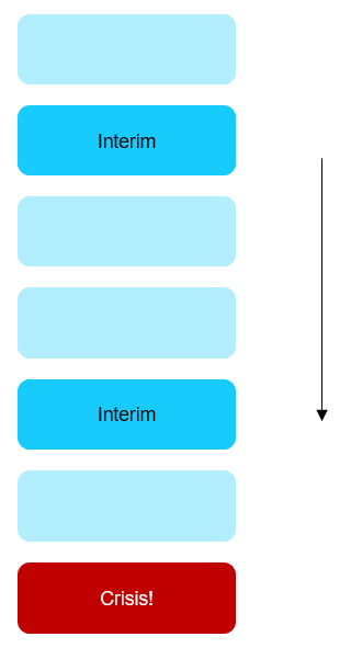
So we have these two types of event:-
Crisis event – what we want to predict, but which we cannot measure
Interim event – what we can measure. It also indicates that the crisis event has not yet happened (as they are mutually exclusive).
The prediction challenge
It is difficult to model and predict customer churn when we cannot see the churn event itself! We don’t know if the customer has lost interest, gone out of business, or simply become less active.
Online customers usually see no downside to a lapse in activity. Contrast this with a telephone contract, say, where we make monthly payments regardless of whether we actually use the service. Order patterns may be due to any number of factors: some customers have standing orders, others order infrequently across varying groups of items etc.
One approach to this problem is to first define and build customer features. We then aggregate them into a customer matrix and add a flag indicating churn (or not). Finally we attempt to map our features to the value of the churn-flag.
Downsides
This poses several problems:
- The definition of churn will be somewhat arbitrary. It may even cause model contamination if we have derived the definition from the same features used to train the model (e.g. average length of time between orders)
- The features will be arbitrary, too. I can begin by taking the sum of orders in the last 30 days, 60 days etc., but we will inevitably lose information when doing this, probably ending up with an inflexible feature set. Should I take the last 87 days, or 321 days: who knows?
- We lose time sequence information: it is a bit like predicting the winner of a football league when 5 games remain. We can aggregate statistics up until the next game (e.g. WWWLW, goals-scored in last 1/5/10 games etc.), but that is no substitute for setting up our model in such a way that it can move through interim events, “seeing” trends peak and then subside. These are details which can get lost when data is aggregated.
- The results from a model built on this data are clear and intuitive to understand, but are also baked into the model itself: i.e. if I have set up the problem to classify customers by using a churn classification (taking one of two possible values: 1 or 0), then that is all I can use once the model has made its predictions: churn prediction – yes or no.
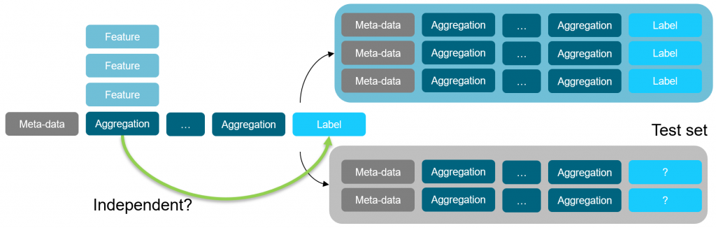
Aggregation overview
Time-to-Event prediction
An alternative way of approaching this problem is not to try and define these elusive crisis events at all. Instead we focus on the interim ones! A prediction as to when the next order will be placed yields an interval, and I can then decide if this interval is significant enough to look like “churn” or not. Or, to put it another way, the customers with the longest predicted TTEs are good churn candidates.
Upsides
It also brings other advantages:
- Each prediction is based on actual historical events (the interim events), rather than on a fictional, contrived event. Remember, we cannot observe the crisis event and so if we are independent of it we will be reducing the amount of guesswork we need to do
- If we treat the problem as a time-series-based one then we can vary the size of batch input at the time of training the model. But we do not have to do this when preparing the datasets (as the batch size is a property of the model, not the dataset)
- The predicted output does not have to be a classification, but can be a distribution. This allows us to choose how we interpret it independently of the model definition
- We can train on censored data
- A TTE can refer to either repeating events (e.g. purchases) or to a one-time “crisis” event (actual churn, where that can be documented, or machine failure). So we can use the same model to apply to both TTE and TTF scenarios
- We can add feedback events (e.g. customer calls, maintenance protocols) to the history. The “group-by-and-aggregate-then-predict” approach is more challenging as it is unclear what other state we have added implicitly to the model
This second approach will use a combination of the following:
- A recurrent neural network (RNN) to process time-series data
- The network outputs two parameters used to define a Weibull distribution
- This distribution is the basis for predicting which entities most likely exhibit the target event in the near future
Censored and uncensored data
We mentioned above that we want to be able to process uncensored and censored data. Uncensored data is a cycle or interval of data that extends up to the crisis/target event. In other words, we can observe a completed cycle; censored data is historical data that is truncated before this event occurs (if, indeed, it ever does). When we move through historical data during the training phase, we can observe censored data before it becomes uncensored, as we are viewing it from a point in time before the subsequent interim event takes place. This means that as we pass through the history, we can review the predictions our model has already made for data which at the time of prediction was still censored: we can penalize predictions that turned out to be “bad” and reward those that proved to be accurate, and we have multiple opportunities to do this.
More about this in part 2, where we will discuss the implementation, technical details and application of a TTE/TTF solution.
N.B. This article and the ideas therein builds on the original theory as first presented by Egil Martinsson:
https://ragulpr.github.io/2016/12/22/WTTE-RNN-Hackless-churn-modeling/
Continue reading part 2 of this post