Predicting hidden events: inverting the time-to-event paradigm: Part 2

Introduction

In part 1 we looked at making a prediction with a time-to-event (TTE) problem, and how to approach this by focusing on interim events. We presented this as an alternative to attempting to identify the crisis – or target – events. In this article we will build on that discussion – so you may find it helpful to read it first!

We ended last time by outlining the following implementation: a recurrent neural network (RNN) that outputs two parameters that we can then use to define a Weibull distribution. Let’s start by looking at that.

A Weibull-tailored implementation of a log-likelihood function is a good fit for censored TTE data (https://en.wikipedia.org/wiki/Weibull_distribution#Standard_parameterization). It can also be used for both discrete and continuous data (and what dataset is truly continuous?). For these reasons we will use it as the output from our neural network.

The network

We will build our neural network using the Keras API with Tensorflow as the backend network implementation. The network will achieve two things:

It uses a custom activation function to allow us to apply more than one activation function to a individual neuron, as we want to output different functions for censored and uncensored data. This is an approach that comes from the field of survival analysis.
It will prepare our data in batch form so that each input is a “look-back” window of data for each step through that data. This will result in batches that are largely overlapping. We will also need to pad them where the sequences are of different lengths.

The prediction distribution

Why the Weibull distribution? Well, we could use a simpler model that simply uses a sliding window. This would output a binary value – do we expect the event in the next window: yes/no? But we cannot use the final window for training as there is no way of knowing if we introduce class imbalance or biases by accepting 1s in the final window, but not 0s, as we can only consider completed event intervals. It is therefore safer to omit the final window.

But we also want the window to be large enough for the results to be actionable (“churn in 60 days?” is better than “churn in the NEXT 10 MINUTES – quick, do something!!!”). If the window is too large we omit too much recent data, so we lose out either way. Outputting a distribution means that we can express uncertainty over an event happening in an as-yet-unfinished event interval.

Secondly, as mentioned above, the Weibull distribution offers both a continuous and a discrete version. This means that we can pre-aggregate data (e.g. by hour, day or calendar-week) as appropriate.

And why use a (black-box) RNN? (as an aside: there are different opinions as to whether neural networks are truly black box models – they do learn patterns that have interpretative meaning, though getting at that information is a challenge).

One clear advantage with an RNN is that we don’t have to spend so much time on feature engineering. The fact that our data is a time-series is explicit – we feed a batch into the RNN, instead of having to “wrangle” it up front.

Application

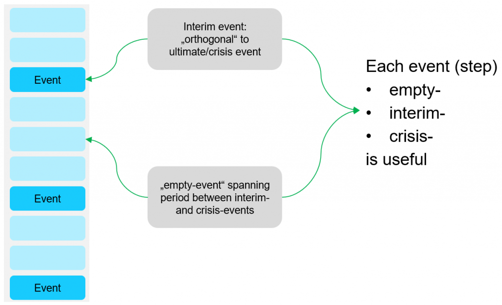
So we now have our data prepared in chronological, overlapping batches. If the data is sparse, then we can simply fill in the “gaps” with what are essentially empty events. The granularity of this will depend on how we have aggregated our batches. But they are still essential as otherwise we would lose information about any time-based trends.

We can feed the batches through the network, one time-step at a time. In the diagram below we show each batch as a block of orange events. As we move (down) through the chronology, we will make a prediction about the next, future interim event. When we actually encounter that event, we can reward or penalize the prediction we have made when processing earlier batches – we represent this with the thumbs up and thumbs-down icons.

We thus have ample opportunity to fine-tune our model while we are training it, and every batch is useful, even ones that are void of interim event information.

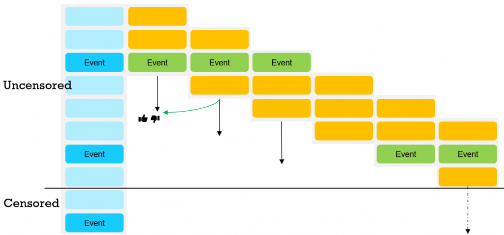
At the bottom of the diagram we have a solid black line that represents the end of the training period. What happens to the final interim event, the one under the line, and the intervening empty events? We call this final period – i.e. all events between the penultimate interim event and the final one under the line – “censored” data.

The Weibull distribution offers a couple of advantages here: the linked article at the bottom of this post explains this in more depth, but essentially the model will take into account how censored the batch is, and distribute the probability across the boundary accordingly.

Interpreting the prediction

The prediction is in the form of two variables, alpha and beta. These define our Weibull distribution so we can alter and redefine the distribution independent of the training phase.

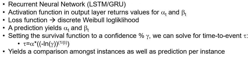
Let’s give an example from customer churn: we can set the confidence level to e.g. 50% and then solve for the TTE given the two variables. This gives us a specific TTE prediction. What does this value mean? If we have a TTE of, say, 10, and we have aggregated our data by week, that would mean that we can have 50% confidence that the next interim event for this customer occurs in 10 weeks’ time. The higher this number, the more “churned” the customer is, since this “10 weeks” may mean one or more of the following:

the customer is no longer active and a burst of activity has long since ceased e.g. weekly orders have trailed off and nothing is expected for roughly the next 3 months
the customer is still active, but they punctuate their activity by long pauses. A long pause may be indistinguishable from “departure”
the customer is still active, but their activity is clearly “tailing off”. We downgrade our prediction of the next event accordingly

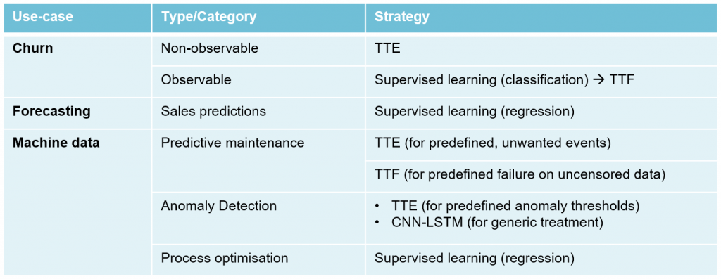
We could give similar examples for other domains, but the principle is the same and can be summarized in the following table:

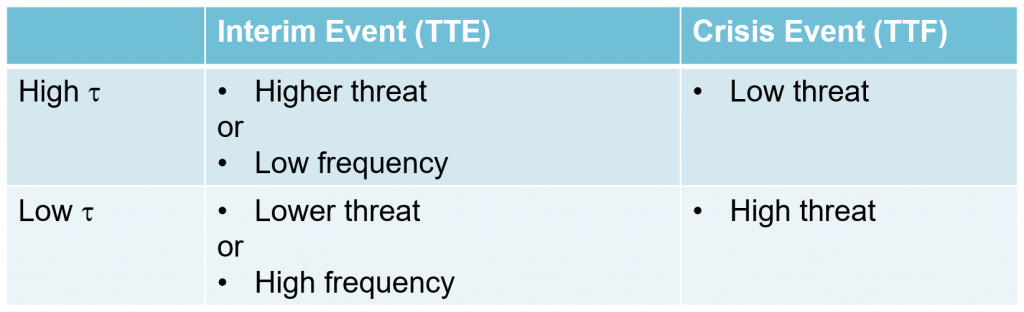
Where would we use this approach? The table below is not exhaustive by any means, but gives an overview of where it (TTE/TTF) may be relevant:

Thank for reading through right to the end! I’ve omitted a lot of implementation detail due to space retraints but you can dig deeper by looking at the following links:

5 2 votes

Article Rating

Introduction

The network

The prediction distribution

Application

Interpreting the prediction

Original thesis – Egil Martinsson (WTTE-RNN)

Optimizations

Other adaptions (Keras, jet-engine analysis etc.)

Definitions

Like this: