Unsupervised anomaly detection using an ensemble of one-class random forest classifiers

Introduction

Unsupervised anomaly detection with unlabeled data – is it possible to detect outliers when all we have is a set of uncommented, context-free signals? The short answer is, yes – this is the essence of how one deals with network intrusion, fraud, and other types of low-instance anomaly. In those scenarios we assume that nearly all of our training data is “’good” (i.e. non-anomalous) and we use a model to analyze it for patterns and trends: we can then use this model with new, unseen data, to identify and flag anything that does not fit the expectations.

In this article I am going to discuss an approach based on two papers. I’ll add a couple of extra assumptions. We won’t spend too long on the underlying theory (the two links provide all the background). Instead we’ll look at how we can implement this with machine data.

Supervised vs. unsupervised training

Just to make this distinction transparent:

• supervised training :- data that is clearly labelled (with a target value or as belonging to a specific class/category)
• semi-supervised training :- data that is partially labelled
• unsupervised training:- data that is not labelled

Setting the scene

We’ll be using data from a Balluff Condition Monitoring sensor. Specifically, temperature and vibration readings in the x, y and z dimensions. At the heart of the approach outlined in the two papers are these two intuitions.

• Firstly, that “the normal data may not have discernible positions in feature space, but do have consistent relationships among some features that fail to appear in the anomalous examples”. In other words, a model uses the other features to predict the target feature. Repeating this for each feature we build an ensemble of predictors – in doing so we have actually trained them to recognise the “shape” inherent in the data as a whole.
• And secondly: “predictors that are accurate on the training set will continue to be accurate when predicting the feature values of examples that come from the same distribution as the training set, and they will make more mistakes when predicting the feature values of examples that come from a different distribution.”

Distortion, not amplitude

As an analogy, imagine two people are out on a tandem bicycle: they can vary their speed, direction and cadence, but whatever they do has to be done in sync with one another! They have degrees of freedom, but only as a unit. If we construct a special tandem bike that can take 4 riders, this will be doubly true! Or imagine a spider’s web: we preserve the shape of the web if we tug on all of the outer nodes of the web in the same way at the same time, but if we just pull on two of them, a distortion of the shape becomes evident.

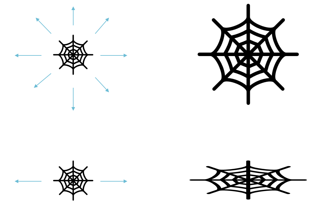
Putting it another way: it may not be sufficient to simply examine how individual features are distributed. We also need to understand the distribution of the relationships between the individual features, so we can recognize those relationships, and identify situations that no longer preserves those relationships.

Combining the results

Having established the general approach, the important question is, how should we weight/combine the individual assessments from each predictor. In the paper, the authors use the error/accuracy (in their case, from the confusion matrix; in our case, that will be something like the mean absolute error), or, more specifically, -log(err). This will be positive number ranging from a low value (interpretation: the model was not a very good predictor, so neither really bad nor really good predictions should say much about its overall correctness) to a high one (interpretation: we expect a consistently high level of accuracy). This is called the surprisal factor, which we will use to weight the predictions from each classifier.

I’ve plotted the distributions of our four values in the following graphs. That of vibration data is, as expected, fairly similar with one strong synchronized peak, together with a second one that varies across vibration dimension.

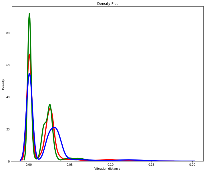
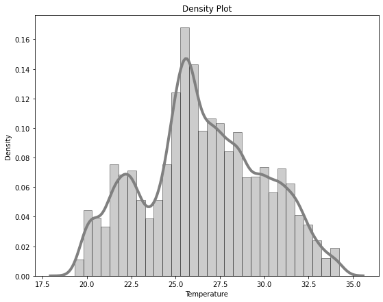
So for this example we have a limited number of features – only 4 – but with 2 very different distributions. We can train 4 models to each predict one feature and then combine their accuracy scores to give a measure of anomaly.

Unsupervised anomaly detection

Before we discuss the implementation, we should briefly consider the second of the two papers mentioned. Our scenario is most likely to be fully unsupervised – i.e. it is not feasible to label all of the training data and we will thus have a mix of anomalous and non-anomalous data in that set, too. So can we still use this approach in an unsupervised way i.e. with completely unlabeled data?

The unsupervised scenario is discussed briefly in section 4 of the second paper, and although tests results show that this approach still performs well, there is no detailed discussion as to why. It seems that the anomalies – which by definition will be sparse – in the training data can be successfully treated as noise i.e. these anomalies are located to a large extent in the training error space (and thus will still “stand out” as outliers in the test data).

Implementation and simplifications

Back to our example: we deploy our models into a microservice environment written in java. For this reason we are a little limited in the modelling frameworks we can use. But we still have strong options to define and train the model:

• Python – and expose the model behind a REST interface (using e.g. python flask)
• H2O – and export and use the model as a java class
• Keras/Tensorflow – and import the model into Deeplearning4j
• Weka – and use the model with Weka java classes

We have chosen the last of these options as Weka gives us flexible options – i.e. for pre-processing our data and comparing different algorithms. The data wrangling steps are as follows:

• Select attributes to avoid too much interdependence
• Define and train models on all features and filter out those with low accuracy
• Make a note of the error metrics and calculate the “surprisal” factor

The result of this data engineering stage was to choose Random Forests for our predictor models. We export each model from Weka and then import them all into our micro service on initialization.

We combined the prediction errors like this (N.B. this is a simplification of the approach described in the papers):

• train models and make a note of model accuracy (A)
• run a prediction on a row and make a note of the actual value (B) and absolute error (C)
• apply log(B) to C giving (D), to weight errors in favor of larger values. This cuts out the distorting effects of noise on smaller values.
• apply A to D to weight errors in favor of those models that were better at predicting on training data
• i.e. overall error = ∑[(model accuracy) * LOG(actual) * ABS(error)]

Further steps

One relative weakness of this approach is that the surprisal consolidation step does a lot of heavy lifting. This is where we combine the individual predictions into an anomaly score – and if we get this wrong, then the results may be misleading.

A simple way to combine these predictions would be to normalize each error, and then apply the surprisal factor. In this way we remove the factors arising from a) different distributions and b) different levels of accuracy.

A further step could then be to discretize the errors over the training set for each model. We distribute them into sqrt(training size) buckets of the same number of similar errors. Smooth this histogram into a gaussian kernel and then extract the probability of a reading landing in a particular bucket.