Improving black-box process efficiency using Bayesian Optimization

Introduction

AutoML (automated machine learning) is one of the recent paradigm-breaking developments in machine learning. New libraries such as HyperOpt allow data scientists and machine learning practitioners to save time spent on selecting, tuning and evaluating different algorithms, tasks that are often very time consuming. Some of these libraries – HyperOpt, for example – use a technique called Bayesian Optimization. Instead of randomly or exhaustively iterating through combinations of algorithms and parameters, the libraries seek to build up an in-memory approximation to the algorithm or process. They then make a selection for the next iteration based on prior knowledge. This is where the Bayesian bit comes in.

As these developments are still in their infancy, it is fair to assume that they are non-trivial in nature. But the underlying mathematics has been with us for about 250 years – thus the complexity more likely lies in the layers of abstraction that make it challenging to measure and compare the accuracy of this approach. The purpose of this article is to look at an approach to macro-tuning  – where an operator has a plethora of machine parameters to configure – that uses Bayesian methods in an identical way.

Setting the scene

This example will be a little contrived in its details, but is based on actual work we are currently doing in the area of smart factories. Imagine that we have robots carrying out a simple function, which can be configured using 6 different parameters. These parameters can take one of 10 discrete values, and influence the process directly. They are things such as torque and power rather than passive measurements such as air humidity.

Assuming zero prior knowledge about recommended settings for these 6 parameters, we will have 10 to the power of 6  – i.e. one million – different combinations to test in order to see which one results in the best immediate efficiency (which is only one measurement of efficiency – more about that later) for our process. Even if the process is rapid, it is just not feasible to work through this using brute force. Neither is it advisable to simple guess at random. Enter Bayesian optimization.

The Bayesian bit

Bayesian theory has a fascinating history, starting in the 1740s with Reverend Bayes throwing objects over his shoulder – or at least, imagining to do so – to see how many landed on the table behind him. The central idea is simple: we have a better idea of predicting the future if we retain information about the past (the “prior” observations).

So far so good. We run our process with a parameter set, measure and record the results and move onto the next attempt. But how does that help us? There are two further parts to our puzzle:

• we will use the prior information to make estimations about the distribution of the process/parameter space, and
• we will have a strategy that directs us to the next parameter set.

Function definitions

We can now lay down some definitions:

• The objective function
  • This is the black-box function that we cannot see. It is the mapping of parameter values to the behavior of our process that we want to optimize
• The parameter hyperplane
  • This is the superset of possible parameter combinations. In our example, it is the 1 million combinations of our 6 discrete parameters
• The surrogate function
  • This is an approximation to the objective function. It is fine-tuned each time we complete an iteration of our process (using the “priors”)
• The acquisition function
  • This is the strategy we use to choose the next candidate from the parameter hyperplane

Before we get more technical, let’s try an analogy. I want to purchase some footwear from Amazon and I have several constraints: the purpose of the purchase, my shoe size, my budget, my personal preference etc. There’s a limit to the amount of trial-and-error orders that Amazon will allow me, so I have to have other ways of “homing in” on that perfect purchase. The obvious solution is to intelligently use the reviews, filtering out the noise and identifying consumers who seem to have similar priorities and goals to my own. Once I have built up a profile of seemingly like-minded customers I can make my purchase based on their recommendation.

This would give us:

• The objective function
  • Buying the perfect footwear for the given purpose
• The parameter hyperplane
  • The constraints on my purchase (size, taste, budget etc.)
• The surrogate function
  • Reviews
• The acquisition function
  • How to filter the reviews

Bayesian optimization: the nuts-and-bolts

Back to our example with the robots – we will keep things simple by assuming we have only a single parameter. Assume we have a univariate function that looks like this:

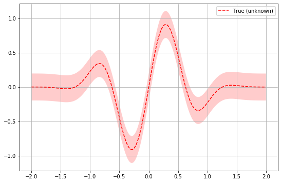
The red line plots a cost metric (Y-axis) against a variable (X-axis) – we can’t see this relationship but it is the one we want to optimize. Typically we will want to minimize this function i.e. find the lowest point on the curve. As we start to iterate through the combinations of parameters settings, we will build up observations (the red dots) that lie on our hidden red line. We can use even a few of these observations to build up a probability distribution (the envelope in green in the diagram below) around an estimated mean (green line). This is our surrogate function. The more observations we have, the better it will approximate to the hidden red line.

We can thus build up on “offline” version of the objective function. We can use it to rapidly examine and sample and to make a guided choice for the next parameter group.

Acquisition strategy

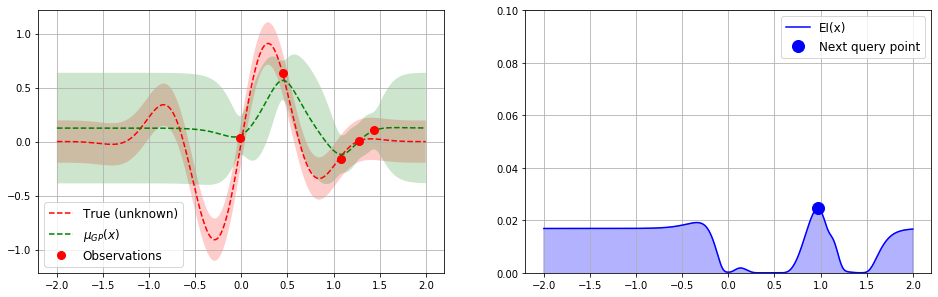
On the right side of the diagram we have our acquisition function. This a strategy function that offers a tradeoff between a) exploiting areas around “good” observations that we have already made, and b) exploring unknown areas far from these observations. We are using “expected improvement” (EI), but there are other candidates such as “upper confidence bound” and “probability of improvement”.

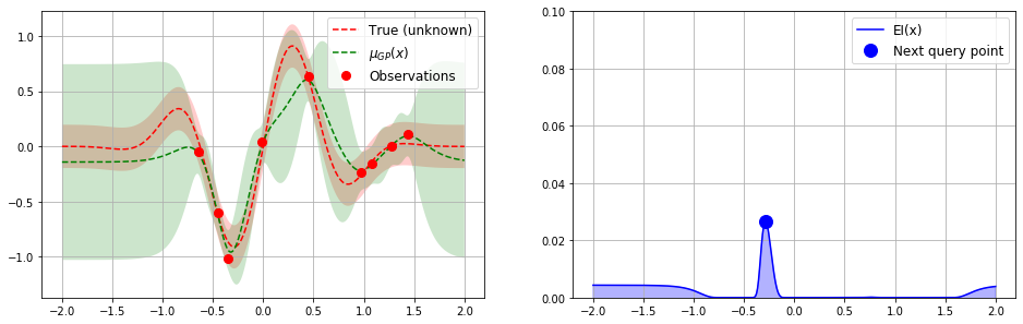
After just a few iterations, the green envelope has collapsed nicely around the hidden function. We can see that we can probably halt the process as the next suggested value from our EI function is very near to the minimum that we have already detected:

Implementation

I said at the outset that this technique is already used in closed-system optimization i.e. processes where we want the optimization to run uninterrupted until a result is issued: for example, parameter tuning during the training phase of model development. However, it is clear that the scenario above is a case of open-system optimization i.e. we call a single optimization iteration once we have run a single batch of our process. This is also known as “ask-and-tell”, and the python machine-learning library scikit-optimize offers an interface to do just this:

https://scikit-optimize.github.io/stable/auto_examples/ask-and-tell.html#sphx-glr-auto-examples-ask-and-tell-py

(I have generated the graphs myself but they borrow heavily from the scikit-optimize example).

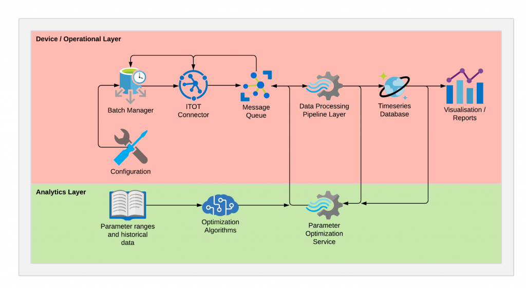
In order to make this functionality available to non-python systems, we will wrap it in a python Flask REST service, which will then be invoked for each batch of our process.

We will also need a batch manager to act as a “conductor”. It will be responsible for applying a given configuration, executing a batch, and then reporting the batch results. We write these results, together with other sensor data that is available, to a message queue. From there they are a) passed to the REST service to collect the next group of parameters settings (our Bayesian optimization service) and b) written to a time-series database and plotted in near-real-time. The following diagram summarizes these steps:

Summary

We have given a brief overview of applying Bayesian optimization methods to black-box processes, showing how to use an ask-and-tell pattern for open-system scenarios. There are some clear limitations to this approach that we should also note:

• Does the black box process map onto any function, or is it purely random?
• Does the black box process map onto the configurable parameters that we have available? Or is it rather influenced by external factors that we cannot directly influence, such as air humidity?
• Is domain knowledge enough to solve our problem? Manufacturers’ recommendations or our own experience may be sufficient.
• Real-time efficiency is only one performance metric. How sustainable is our process and are we prioritizing speed over long-term maintenance issues?

One last point: in contrast to many other machine learning scenarios we need very little data to perform Bayesian optimization; just our parameter hyperplane and a few initial observations, and off we go!